Conditional Formatting in Excel

Introduction

This article is written over Excel conditional formatting. This is very useful when we are working on large volume of data. We can separate data as per our circumstances. I am here explaining in detail how to mark duplicate data or specific type. Here is as follow:

Step 1: Launch your Excel through shortcut (Windows + R) or launch through program files.

                   



Step 2: Select range where you need to provide conditional formatting in excel sheet.

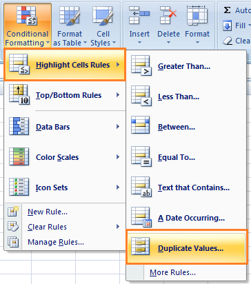
Step 3: On Home menu, there is an icon containing conditional formatting, now drill down conditional formatting menu.

Step 4: Now expand sub menu Highlight Cell Rules, then expand more sub menu Duplicate Values…, now click on it.

                                  

Step 5: Now a popup window will pop up Duplicate Values, Now drill down drop down list, select Duplicate from the list and right side click on values with list, now next select Light Red Fill with Dark Red Text, and click finally on OK button.

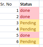
Step 6: Now on this step, you may check status column, where duplicate is populated light red after conditional formatting.

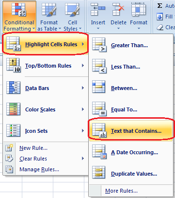
Step 7: Now again another one more formatting of specific word Working is conditional formatting. In the same way above steps, expand Highlight Cell Rules, then expand sub menu Text that Contains…

                                   

Step 8: Now again a window will popup Text That Contains, now type in text box Format cells that contains the text, in this example Working is typed here, now drill drop down list with, select Green Fill with Dark Green Text, then finally on OK button.

Step 9: Now you can see in the picture where Duplicate, & on specific words conditional formatting is done.

                                   
  

Conclusion

Excel work is very essential to our daily routines work, whenever we are dealing with data volume, analyzing data or put data in systematic way, then conditional formatting plays a vital role in manipulating data. 

Video: Conditional Formatting in Excel